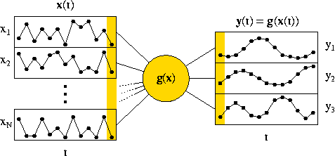
Slow feature analysis

Slow feature analysis (SFA) is an algorithm for extracting slowly varying features from a quickly varying signal (see Figure 1).

Figure 1: Illustration of the optimization problem solved by slow feature analysis.

The optimization problem can be formulated as follows. Given a vectorial input signal x(t), find an input-output function g(x) that generates a vectorial output signal y(t) = g(x(t)) with the following properties:

• The output signal should vary slowly, i.e.
  • the variance of the time derivative is minimal: minimize <(d y_i / dt)²>.
• The output signal should carry much information, i.e.
  • y_i has zero mean: <y_i> = 0,
  • y_i has variance 1: <y_i²> = 1
  • y_i and y_j are uncorrelated: <y_i y_j> = 0 for all j < i.

Slow feature analysis solves the optimization problem given above if the input-output function is constrained to lie within a finite dimensional function space, e.g. if it is a polynomial of some fixed degree. In that case the otherwise very difficult problem of variational calculus can be solved easily as is illustrated in Figure 2.

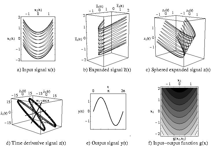
Figure 2: Illustration of the slow feature analysis algorithm. (a) A two-dimensional input signal is given. It rocks back and forth on a parabola, which moves slowly up and down. The slow sinosoidal up-and-down motion is the slow feature to be extracted. (b) If we confine the input-output function to be a polynomial of order two, the first step is a non-linear expansion into the space of all first and second degree monomials. In that five-dimensional space the problem is linear. Only three of the five dimensions are shown here. (c) The next step performes a normalization (sphering or whitening) so that the signal has zero mean and unit variance in all directions. Furthermore, two orthogonal directions are uncorrelated. Thus the zero mean, unit variance, and decorrelation constraints are fulfilled by any orthogonal set of directions. Thus the only job that remains to be done is to find the directions of minimal variance of the time derivative. (d) In order to find these direction the time derivative of the normalized signal is computed. It is clear that the time derivative signal has little variance in the direction of slwo variation, resulting here in the flat eight-shape. Thus the eigenvectors belonging to the smallest eigenvalues are the directions we are looking for. In this example only one eigenvector is relevant. (e) If we project the signal of (c) onto the last eigenvector (with smallest eigenvalue) in (d), then we get the slow feature signal shown in (e) which we were looking for. (f) Putting all the steps together results in the effective input-output function g(x), which is only one-dimensional here. For higher-dimensional input-output function more than one eigenvector must be used.